Liquidity position

Last modified: April 22, 2026

Consider a CenturionDEX v3 liquidity pool with tokens $X$ and $Y$. Throughout this section, the price will always mean the price of token $X$ expressed in units of token $Y$. Suppose that a liquidity provider chooses to supply liquidity over the price interval $[p_a,p_b]$. We adopt the convention that the position is active on the closed interval $[p_a,p_b]$. The defining feature of CenturionDEX v3 is that the position is active only within that interval: its liquidity is used to facilitate trades only while the market price remains between $p_a$ and $p_b$. If the price moves outside the chosen range, the position becomes inactive and its balances remain unchanged until the price re-enters the interval $[p_a,p_b]$. Moreover, if the price falls below $p_a$, the position is entirely converted into token $X$; if the price rises above $p_b$, it is entirely converted into token $Y$. In other words, once the price exits the range, the position ends up holding only the token associated with that side of the interval.

Although the CenturionDEX v3 AMM still relies on a constant-product structure, the geometry must be modified so that one of the token balances can become zero exactly when the price reaches one of the interval boundaries. To achieve this, we apply the translation illustrated in the animation below to the virtual constant-product curve

where $(x_v,y_v)$ denote virtual reserves; we will distinguish these from real balances $(x,y)$ below.

Recall that, for a state $(P=(x_v,y_v))$ on this virtual curve, the price is given by

which is precisely the slope of the line joining the origin to $P$. Consequently, in the animation above, the state $a$ corresponds to the lower boundary price $p_a$, while the state $b$ corresponds to the upper boundary price $p_b$, and therefore $p_a<p_b$.

To determine the translation that converts the virtual constant-product curve into the actual balance curve of a CenturionDEX v3 position, we begin by evaluating the virtual boundary states associated with the chosen price interval $[p_a,p_b]$. Let

denote the virtual states corresponding to the lower and upper boundary prices $p_a$ and $p_b$, respectively. Since these states lie on the virtual curve

and satisfy

we obtain

and

Therefore,

At the lower boundary $p_a$, the actual balance of token $Y$ must be zero, so the corresponding real state must lie on the horizontal axis. This requires a downward translation by $L\sqrt{p_a}$. Likewise, at the upper boundary $p_b$, the actual balance of token $X$ must be zero, so the corresponding real state must lie on the vertical axis. This requires a leftward translation by $L/\sqrt{p_b}$. Hence, the virtual curve is translated by the vector

Applying this translation to the virtual curve $x_v y_v=L^2$, we obtain the equation of the real-balance curve:

This is the curve of real balances shown in the animation above.

Applying the same translation to the boundary virtual states yields the corresponding real boundary states

These are precisely the two endpoints of the active range on the real-balance curve.

Virtual reserves. We now introduce the virtual reserves, which are central to the concentrated-liquidity model. Let $x$ and $y$ denote the actual balances of tokens $X$ and $Y$ in a position, and let $x_v$ and $y_v$ denote the corresponding virtual reserves. By definition, the virtual reserves satisfy the constant-product relation

and the spot-price relation

where $p$ is the current price of token $X$ in units of token $Y$. Thus, $(x_v,y_v)$ represents a virtual pool state lying on the virtual curve in the animation above. When the market price remains inside the interval $[p_a,p_b]$, trades are modeled as taking place along this virtual constant-product curve, even though the actual balances of the position are given by the translated real-balance curve.

The real and virtual reserves are related by the translation derived above:

Accordingly, the real-balance equation above may be written equivalently as

or, in virtual-reserve form,

Since

it follows that

Real balances at price $p$. We can now express the actual balances of a position as functions of the current price. If $p\in[p_a,p_b]$, then the position is active and the real-balance equation above applies. Substituting the virtual-reserve identities above into the translation relation, we obtain

In the boundary cases, these formulas reduce to the expected values. If $p=p_a$, then

so the position is entirely held in token $X$. If $p=p_b$, then

so the position is entirely held in token $Y$.

If the price moves outside the active interval, the balances remain frozen at the nearest boundary state. Therefore, the actual balances of a CenturionDEX v3 position are given by the following piecewise formulas:

This is the natural canonical piecewise form.

Opening a position. Suppose now that a liquidity provider wants to create a CenturionDEX v3 position with chosen parameters $p_a$, $p_b$, and $L$. Since trading fees in CenturionDEX v3 are accounted for separately rather than automatically reinvested into liquidity, the parameter $L$ remains fixed for a given position unless liquidity is explicitly added or removed. Consequently, once $p_a$, $p_b$, and $L$ are fixed, both the virtual-balance curve and the real-balance curve are fixed as well, and the state of the position always lies on the corresponding real-balance curve.

It follows that, given the current price $p$, the liquidity provider must deposit exactly the token amounts prescribed by the piecewise formulas above. Concretely, there are three possible cases.

(i) If the current price satisfies $p<p_a$, then the position starts entirely in token $X$. The required deposit is

(ii) If the current price satisfies $p_a\le p\le p_b$, then the position starts with both tokens. The required deposits are

(iii) If the current price satisfies $p>p_b$, then the position starts entirely in token $Y$. The required deposit is

These three situations correspond to the three states represented in animation below.

Example

In practice, a liquidity provider will usually not choose the liquidity parameter $L$ directly. Instead, the provider selects a price interval $[p_a,p_b]$ and decides how much of one of the two tokens to contribute. Once that information is fixed, the value of $L$ can be recovered from the position formulas, and the required amount of the other token can then be computed accordingly.

Consider a CenturionDEX v3 pool between CTN and USDC, and suppose that the current price of CTN in units of USDC is

Assume that a liquidity provider wants to open a position over the interval

and that, at the current price $p_0$, they want the position to contain

units of CTN.

Since $p_a < p_0 < p_b$, the position is opened inside its active interval, so both tokens must be deposited. From the canonical formula for the real balance of token $X$ inside the active range, we have

Evaluating at $p=p_0$, we obtain

Hence,

Now that $L$ is known, the required amount of USDC follows from the canonical formula for the real balance of token $Y$ inside the active range:

Therefore,

Thus, to open the position, the liquidity provider must deposit

Value of a Position

We now compute the value of a CenturionDEX v3 position as a function of the current price. Let $x(p)$ and $y(p)$ denote the real balances of tokens $X$ and $Y$ held by the position when the price is $p$. The value of the position, expressed in units of token $Y$, is

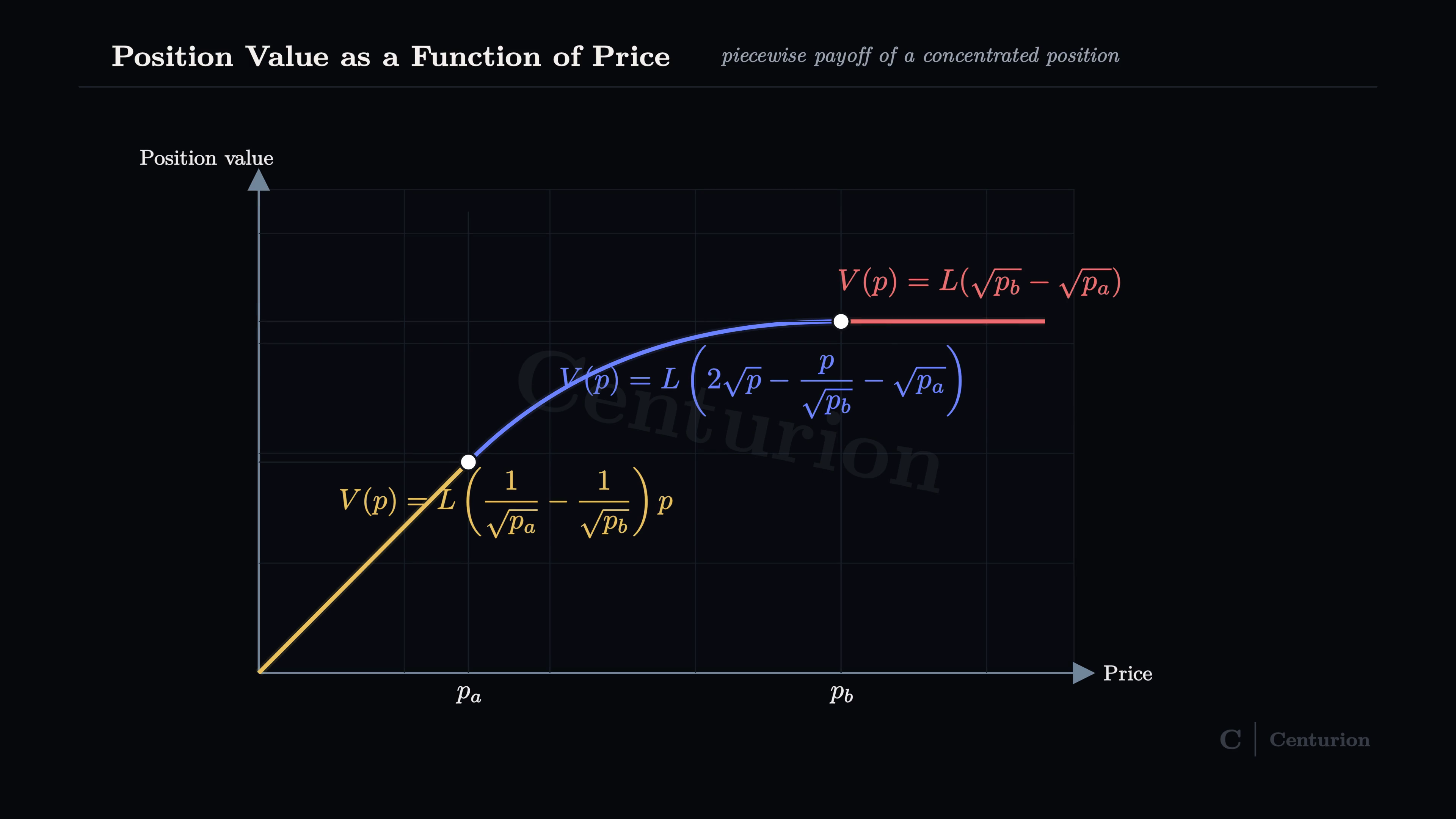
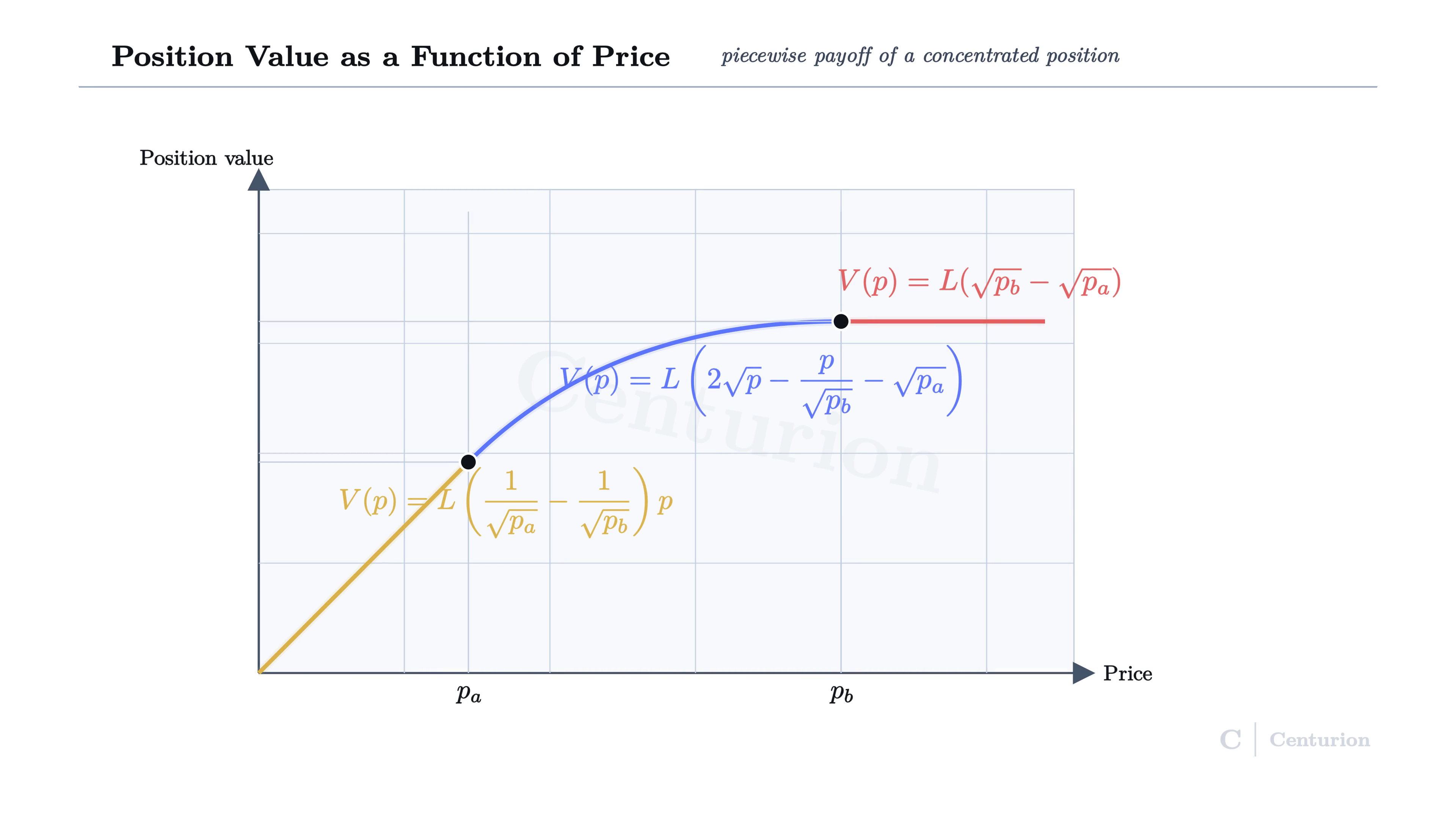
Once a position is created, the parameters $L$, $p_a$, and $p_b$ are fixed. Using the canonical balance formulas, we obtain the following piecewise expression for the position value.

If $p \le p_a$, then the position is entirely held in token $X$, so

If $p_a \le p \le p_b$, then the position holds both tokens, and therefore

After simplification, this becomes

Finally, if $p \ge p_b$, then the position is entirely held in token $Y$, and hence

These formulas describe the value of the position throughout the entire price range and are the basis for the plot shown below.

Worked example

Consider the position constructed in the example above. Its parameters are

and it was opened at price

with deposits of $5$ CTN and $21000$ USDC. Therefore, the initial value of the position is

Now suppose that the price rises to

Since $2500 < 4225 < 4900$, the position remains inside its active interval, so both balances must be recomputed using the in-range formulas. The CTN balance becomes

The USDC balance becomes

Hence, the value of the position at the new price is

Now compare this with the value the liquidity provider would have had if they had simply held the original assets outside the pool. In that case, the portfolio would still consist of $5$ CTN and $21000$ USDC, whose value at price $4225$ would be

Since

the liquidity provider is worse off than under simple holding. The difference is

which is the impermanent loss associated with this price move.

We will analyze impermanent loss in CenturionDEX v3 in more detail in the next section.